Euler's Formula 2 - Going in Circles
Euler's Formula (2 of 2)
So let’s start from the other side of Euler’s formula, the part that is about circles, and go through the whole shebang in the opposite direction from the very basics.
When measuring distances travelled around the circumference of a unit circle we define the number  to be the length of half a circumference, so the length of the circumference of a unit circle is
 . Travelling around a unit circle, distances are equivalent to angles. By convention we always begin measuring the angle from the horizontal axis and moving in the anticlockwise direction. In the diagram from last time the angle
 happens to be
 , the same as
 .
If you’re wondering why we only measure the distance halfway around the unit circle and make that the unit of angle, you ain’t the first. It was an arbitrary choice, and was originally defined as the ratio between the circumference and the diameter, and a unit circle has a diameter of  , so only gets you halfway. As a result we are doomed to say in a lot of formulae.
Sine and Cosine
Given an angle, it is surely possible to compute the  coordinates of the corresponding point on the circumference of the unit circle. There must exist a pair of functions that give these coordinates, and they are:
-
 (“sine”) gives the vertical or
 coordinate, and
-
 (“cosine”) gives the horizontal or
 coordinate.
Without knowing anything else about these functions, we can already see that as an object progresses around the circle, its coordinates must visit these milestones:
- We begin at
 , the right-most point of the circle, where
 and
 .
- At
 (90
 ), the top of the circle, the situation has reversed:
 and
 .
- At
 (180), the left-most point of the circle, and
 .
- At
 (270), the bottom of the circle,
 and .
We can plot by itself between the values  and (actually I started a little bit before so you can see how it repeats), and likewise .
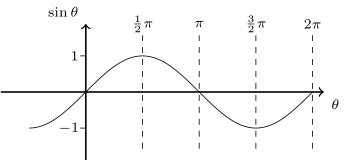
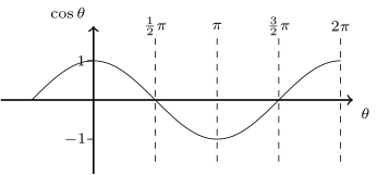
We can see that  is just
 slid along to the left by a quarter of a cycle, so it “runs ahead” of :

If we advanced by , half a cycle, the peaks and valleys would change places, while the uphill slopes that cut through the horizontal axis would become downhill slopes and vice versa. In other words, it would look exactly like we’d flipped the function upside down:
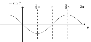
So:

Incidentally, the word cycle is from the Greek word for circle. The word phase is also used a lot in this context, probably deriving from the phases of the moon. When one periodic function is equal to another shifted by some amount, we say there is only a phase difference between them.
Differential Calculus on Sine and Cosine
It’s interesting how much we can figure out intuitively before we even have a way of computing these functions. Here I’m going to assume we know that velocity is the rate of change of displacement.
Think of an object moving along the unit circle’s edge at a constant rate, one unit of distance per unit of time, so its velocity vector is a unit vector, just like its displacement vector. At any instant that velocity vector,  , is pointing along the tangent, but this is always at a right angle to the displacement vector,
 , which is the line segment reaching from the centre to the object (the radius).
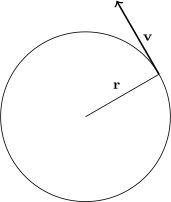
The velocity vector is therefore fixed to be a quarter cycle ahead of the displacement vector, which is precisely the relationship between and . The components of are the rates at which the corresponding components of change as the angle advances. It follows that the rate at which is increasing is given by , or:
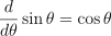
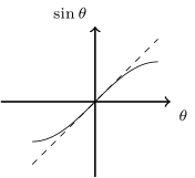
This is confirmed by examining the shape of the functions separately. Nearby to , is closely approximated by itself, and looks much like a straight line of gradient  , which happens to be the value of
 .
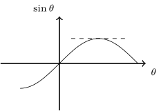
When peaks at , its gradient is , and again this is in agreement with the value of  . This pattern continues at every point in the cycle.
So in any situation where we need the derivative of , we just replace it with . By the same reasoning (and because we know the same relationship exists between  and ) we can assume that:
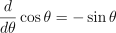
Differentiating two more times will get us back to because each differentiation advances the function by a quarter cycle. (Naturally integration performs the same trick in the opposite direction, but we aren’t going to need that here.)
Computing Sine and Cosine
Now we can take the derivative of , also the derivative of the derivative, and so on, and we know all their precise values at , we can use the Taylor series method (actually the simpler form of it called a Maclaurin series) to find how to compute using only addition and multiplication, if only we have the patience to perform an infinite sequence of those operations.
We begin by assuming that a function  can be expressed as the sum of an infinite series of polynomial terms, that is, each term is some constant
 multiplied by the variable raised to an integer power
 , beginning at :

Anything raised to the power of is , and raising something to the power of makes no difference, so at the expense of consistency, and meanwhile also sneaking in the name of the function we want to compute, we just write:

So we only need to determine the constant factors to entirely characterise the function (does this mean that functions are vectors? Well, yes, the ones that are amenable to being defined in this way, which is actually not all functions.)
Setting  , any term that is multiplied by must be zero (they vanish entirely from the sum), which only leaves
 . But
 , so it follows that
 . We got one of the launch codes!
The next step is going to involve assuming another bit of knowledge: how to get the derivative (the “rate of change”) of a polynomial. Taking the derivative of both sides (so becomes , as we already figured out):

Each polynomial’s power is reduced by , and the original power “moves down” to become an extra factor. Now the exact same vanishing argument applies to  except that here it is solely responsible for the value of
 , and so it must be that
 . We differentiate a second time:

So  . Differentiate a third time:

So  . When is even the term is zero, and when is odd the term
 is divided by the accumulated value
 . We continue in this fashion to find that:

By the same process we find that for only the even- terms appear in the result:

In each case there is a four stage cycle, with alternating absence of terms and then similarly alternating  /
 signs. We saw these exact patterns last time in the result we got from the binomial expansion of the compound interest formula:

Even if we hadn’t already seen that, we might have found it curiously reminiscent of the cyclic behaviour of  .
The exponential function  has the useful property that its derivative is , i.e. the function is its own derivative. But even if we’d only heard a rumour of this, we could confirm it easily, because the method of evaluating at zero and taking repeated derivatives becomes ridiculously easy to perform, and yields:

This is exactly what we got from the compound interest formula, and so we now have two ways of arriving at:

Physics is thick with examples of oscillation. To describe the state of a particle undergoing simple harmonic motion along a line, we need to know the position and the momentum. A snapshot of an oscillator at one moment does not give us a complete understanding: the oscillator might be passing through the origin, but which way?
A complex number, being described by two real numbers, can encapsulate both these quantities, and the real and imaginary parts have the right phase relationship to represent the position and the momentum.
Most importantly, that sense of the inherent weirdness, a feeling of “Yeah, but what does that mean?” when we see some exotic object (such as a linear operator) being used as the power to raise to, is fully banished by the Taylor expansion or the binomial expansion that produces the same result. They show us exactly how to convert  into a sum of terms in which the exotic object is merely the base instead of the power, and the power is just an ordinary number. We only need to know how to multiply the exotic object by itself.
Not yet regretting the time you've spent here?
Keep reading: