Quantumania 22 - Three Dimensions

When we first looked at the Hadamard gate there arose three matrices representing directions in physical space. They were introduced a little abruptly like background characters in someone else’s story, and they deserve some more spotlight. Here they are again:

Z = \begin{bmatrix} 1 & 0 \\ 0 & -1 \end{bmatrix} \quad X=\begin{bmatrix} 0 & 1 \\ 1 & 0 \end{bmatrix} \quad Y=\begin{bmatrix} 0 & -i \\ i & 0 \end{bmatrix}

Geometrically they are all simply reflections. This is most obvious in $Z$ , because they’re all written in the $Z$ basis. $Z$ just flips the sign of the second coordinate (the one that scales $\ket{1}$ ) and has no effect on the first coordinate (the one that scales $\ket{0}$ ). Or to put it another way, a vector of the form $c\ket{0}$ , where $c$ is any complex scalar, is entirely unaffected:

Z c\ket{0} = c\ket{0}

whereas a vector of the form $c\ket{1}$ experiences a sign-flip:

Z c\ket{1} = -c\ket{1}

So these, being only scaled by $Z$ , are the eigenvectors of $Z$ , whereas any other vectors will not only be scaled, they will be re-aligned. In general any state vector $\ket{\psi}$ can be written:

\ket{\psi} = a\ket{0} + b\ket{1}

The probability of measuring state $\ket{0}$ is $aa^* = |a|^2$ , and for $\ket{1}$ it’s $bb^* = |b|^2$ . But the act of multiplying (say) $a$ by its own complex conjugate has the effect of erasing any overall complex phase, because:

\left( e^{i\theta} \right)^* = e^{-i\theta}

and:

e^{i\theta}e^{-i\theta} = e^{i\theta-i\theta} = e^0 = 1

This means that although $Z$ flips the sign of $\ket{1}$ , this does not constitute an effect on anything physically significant about the state, because a sign flip is just a phase factor.

The other matrices represent the two orthogonal directions to $Z$ . $X$ swaps the coordinates between $\ket{0}$ and $\ket{1}$ , performing a reflection around the $45^\circ$ line lying between them. This is the line that $\ket{+}$ sits on (if you’ve read the previous entries, you’ll be familiar with the diagram by now.) So $Z$ has no effect at all on $\ket{+}$ , meaning that here $\ket{+}$ plays the same role that $\ket{0}$ played under $Z$ . Likewise, a vector aligned with $\ket{-}$ would flip to point the opposite way. So if we were to rewrite all these matrices in the $X$ basis, then the $X$ matrix would have that same simple $\operatorname{diag}(1, -1)$ form that we’ve given to the $Z$ matrix.

$Y$ is apparently the most exciting, in that it seems to combine both ingredients seen so far: a sign difference between the coordinates (like $Z$ ) and a swapping between the coordinates (off-diagonal entries only, like $X$ ), but to these it adds an overall factor of $i$ . Again we can see how it affects its eigenvectors, which are given the mnemonic labels $\ket{+i}$ and $\ket{-i}$ to remind us of the coordinate on $\ket{1}$ :

\ket{+i} = \frac{\ket{0} + i\ket{1}}{\sqrt{2}} \quad \quad \ket{-i} = \frac{\ket{0} - i\ket{1}}{\sqrt{2}}

Visualising this geometrically at first seems next to impossible (the $\ket{1}$ component has been scaled by a complex rotation that nevertheless doesn’t change its alignment), but based on the pattern so far, we’d expect $Y$ to have no effect on $\ket{+i}$ (we can ignore the overall $\frac{1}{\sqrt{2}}$ because it appears on both sides of the equation):

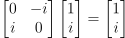
\begin{bmatrix} 0 & -i \\ i & 0 \end{bmatrix} \begin{bmatrix} 1 \\ i \end{bmatrix} = \begin{bmatrix} 1 \\ i \end{bmatrix}

Check! Whereas it should perform an overall $-1$ scale on $\ket{-i}$ :

\begin{bmatrix} 0 & -i \\ i & 0 \end{bmatrix} \begin{bmatrix} 1 \\ -i \end{bmatrix} = \begin{bmatrix} -1 \\ i \end{bmatrix} = - \begin{bmatrix} 1 \\ i \end{bmatrix}

All is as expected. In fact we can visualise it geometrically if we just relabel the axes on our usual diagram (come on, it’s been a while). When we use the $Z$ -basis unit vectors $\ket{0}$ and $\ket{1}$ to express the eigenvectors of $X$ , we quietly ignored $Y$ , leaving it off the diagram. Well, now we can switch allegiance:

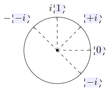
What is this voodoo?! Actually we’re still technically in the $Z$ -basis here, because our vertical axis $i\ket{1}$ is just as much of a valid eigenvector of $Z$ as is $\ket{1}$ . Our diagrams have to be real subspaces of $\mathbb{C}^2$ . We normally draw the real subspace spanned by $\lbrace \ket{0}, \ket{1} \rbrace$ , now we’re using the real subspace spanned by $\lbrace \ket{0}, i\ket{1} \rbrace$ .

In Bloch sphere terms, it gets even simpler. First, think of the usual $\lbrace \ket{0}, \ket{1} \rbrace$ diagram. It is easily visualised as a circular slice through the Bloch sphere (with one important caveat). If you follow a point moving around that circle, it visits $\ket{0}$ , $\ket{+}$ , $\ket{1}$ , $\ket{-}$ in that order. Or to use their physical-space names instead of computing names, $\ket{u}$ (up), $\ket{f}$ (front), $\ket{d}$ (down), $\ket{b}$ (back):

The Bloch sphere with the X-Z circular slice highlighted, visiting |0>, |+>, |1>, |->

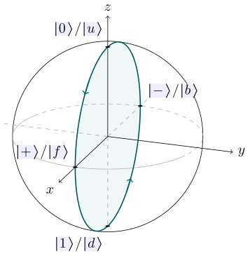
There is no way to access $\ket{l}$ (left) $\ket{r}$ (right) from the provided ingredients if you are restricted to using only real coordinates to scale them. It’s the $X$ - $Z$ great circle, no $Y$ ingredients are supplied, so the rest of the sphere is out of bounds. The caveat I mentioned is that the circle on the flat state space diagram is not precisely the same circle as this slice through the Bloch sphere, because $\ket{0}$ and $\ket{1}$ are orthogonal in the state space, whereas in the corresponding Block sphere great circle they are antipodes (on opposite sides). The angle separating any two states is doubled on the Bloch sphere.

Now with $\lbrace \ket{0}, i\ket{1} \rbrace$ as the axes of our state space diagram, we can access a great circle that visits $\ket{0}$ , $\ket{+i}$ , $i\ket{1} \propto \ket{1}$ , $\ket{-i}$ , or $\ket{u}$ , $\ket{r}$ , $\ket{d}$ , $\ket{l}$ , never $\ket{f}$ or $\ket{b}$ . It’s $Y$ - $Z$ only, and has no $X$ ingredients for us to scale with our strictly real coordinates:

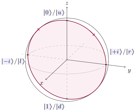
The Bloch sphere with the Y-Z circular slice highlighted, visiting |0>, |+i>, |1>, |-i>

Note how the state diagram’s $i\ket{1}$ only differs by a phase factor ( $-1$ ) from $\ket{1}$ , so these refer to the same point on the Bloch sphere.

We’ve still only scratched the surface of this topic. For example, the matrices are reflections in 2-dimensional complex state space. What are they in the Bloch sphere, that is, in real 3-dimensional physical space?

Not yet regretting the time you've spent here?