Quantumania 13 - The Hadamard Gate

So Hermitian operators represent observables, and their eigenvectors are post-measurement orthogonal vectors, who eigenvalues are the measurement results. That is, if you apply the operator to a unit eigenvector, it will be scaled by an eigenvalue that tells you what the measurement result would be if the state vector was exactly that eigenvector.

When measuring the state of a qubit along Z, the possible results are $+1$ and $-1$, and so we can pack these into a diagonal matrix $\operatorname{diag}(1, -1)$, and that is the Hermitian operator for the observable “measure along Z”, expressed in the Z basis.

But one direction is no different from another: space is symmetrical like that. So there must be similar matrices for the other two spatial directions, but still expressed in the Z basis. If we expressed them in the X basis, then the Hermitian matrix for X would be $\operatorname{diag}(1, -1)$. Switching the basis to another one of these canonical directions can often just mean switching the labels between the same matrices. Expressed in the Z basis then, they are:

\[Z = \begin{bmatrix} 1 & 0 \\ 0 & -1 \end{bmatrix} \quad X = \begin{bmatrix} 0 & 1 \\ 1 & 0 \end{bmatrix} \quad Y = \begin{bmatrix} 0 & -i \\ i & 0 \end{bmatrix}\]

So remember that the X and Y matrices are really the same as Z, but applied inside a “unitary sandwich”, $UZU^\dagger$. So as we can see Z is essentially a reflection, flipping the sign of the $\vert d \rangle$ coordinate, so must the other two be, just disguised by being expressed in a foreign basis. In geometrical terms, they’re the same operator twisted to act in different directions (technical term: “unitarily equivalent.”)

Now, here the letters used for standard things are unfortunately going to get egregiously confusing, as they so often do. I’ve been using $U$ to stand for any unitary operator, and $H$ for whatever hermitian operator. But there is a super handy unitary operator named after Jacques Hadamard, and tempting as it is to call it $J$, I’m going to have go with normal practice and label it $H$ (and try to avoid using that to stand for any hermitian operator from now on):

\[H = \frac{1}{\sqrt{2}} \begin{bmatrix} 1 & 1 \\ 1 & -1 \end{bmatrix} = \begin{bmatrix} \frac{1}{\sqrt{2}} & \frac{1}{\sqrt{2}} \\ \frac{1}{\sqrt{2}} & -\frac{1}{\sqrt{2}} \end{bmatrix}\]

Fortunately it is hermitian, as well as unitary! These are not mutually exclusive categories. Where both apply:

\[H = H^\dagger = H^{-1}\]

Unitary means that its conjugate transpose is its inverse, and hermitian means it is its own conjugate transpose. So an operator that is both therefore must be its own inverse. Apply it twice and you get back to where you started.

The role it’s playing here is not a QM measurement operator, but a unitary transform corresponding to a $90^\circ$ rotational change of basis in physical space. If we sandwich it around Z matrix, we get the X matrix:

\[\begin{eqnarray*} HZH^\dagger &=& HZH \\ &=& \begin{bmatrix} \frac{1}{\sqrt{2}} & \frac{1}{\sqrt{2}} \\ \frac{1}{\sqrt{2}} & -\frac{1}{\sqrt{2}} \end{bmatrix} \begin{bmatrix} 1 & 0 \\ 0 & -1 \end{bmatrix} \begin{bmatrix} \frac{1}{\sqrt{2}} & \frac{1}{\sqrt{2}} \\ \frac{1}{\sqrt{2}} & -\frac{1}{\sqrt{2}} \end{bmatrix} \\ &=& \begin{bmatrix} \frac{1}{\sqrt{2}} & \frac{1}{\sqrt{2}} \\ \frac{1}{\sqrt{2}} & -\frac{1}{\sqrt{2}} \end{bmatrix} \begin{bmatrix} \frac{1}{\sqrt{2}} & \frac{1}{\sqrt{2}} \\ -\frac{1}{\sqrt{2}} & \frac{1}{\sqrt{2}} \end{bmatrix} \\ &=& \begin{bmatrix} 0 & 1 \\ 1 & 0 \end{bmatrix} \end{eqnarray*}\]

But as it is its own inverse, if we do the same sandwich trick with the X matrix, we get back to the Z matrix. It flips between the two. We can interpret this as either a transformation we can apply to a state vector, or a change of basis that takes us between the Z and X bases. It’s yet another a chance to admire our favourite diagram:

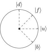
Sometimes it’s said that $H$ works like a combination of a $45^\circ$ anticlockwise rotation, followed by a reflection around the axis that the $\vert f \rangle$ vector lies on. To see how this explanation works, first start with $\vert u \rangle$:

• rotate it $45^\circ$ anticlockwise, now it’s $\vert f \rangle$,
• reflect it around $\vert f \rangle$, that has no effect on it, so the final result is $\vert f \rangle$.

Then start with $\vert d \rangle$:

• rotate it $45^\circ$ anticlockwise, now it’s pointing the opposite direction to $\vert b \rangle$,
• reflect it around $\vert f \rangle$, that flips it around to $\vert b \rangle$.

So $\vert u \rangle$ becomes $\vert f \rangle$, while $\vert d \rangle$ becomes $\vert b \rangle$. Then try going the other way - start from $\vert f \rangle$:

• rotation takes us to $\vert d \rangle$,
• reflection goes back to $\vert u \rangle$.

And finally from $\vert b \rangle$:

• rotation takes to $\vert u \rangle$,
• reflection to $\vert d \rangle$.

How does it achieve these miracles? What, fundamentally, is it, in geometrical terms? For the three observable direction matrices X, Y and Z, we know they are fundamentally all the same thing: a simple reflection. The only difference is that they’ve been sandwiched between some unitary rotation “bread”… wait a second!

Could it be that $H$ is also unitarily equivalent to $Z$? Yes it could. All four of these matrices are geometrically the same thing: a reflection, just aligned along different axes.

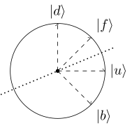
Look how ridiculously simple it actually is: just pure reflection around that dotted line on the $\pi/8$ axis, bisecting the angle between $\vert u \rangle$ and $\vert f \rangle$.

There are good reasons for sometimes thinking of it as a rotation by $\pi/4$ followed by a reflection around the $\pi/4$ axis, one of which is that the implementation of this operation in a quantum computer may be composed of successive operations in exactly that way.