Quantumania 10 - Adventures of Stick Man

It’s high time we looked at linear operators in a bit more detail, so we can get a feel for how they work, and maybe categorise them a bit. To start with we’ll pretend scalars are real numbers, and we’ll work in the plane, that is, two dimensions. This is probably going to seem like a massive digression but it will be fun, and I promise it is highly relevant to QM (eventually.)

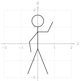
Oh look, it’s Stick Man. Doesn’t he seem friendly? But what does he have to do with vectors? Think of each point on the figure as being related to a vector that reaches from the central origin to that point. In that sense, the drawing is described by vectors. We can represent each point with a coordinate pair, which is the column vector for that point in our basis, that basis being the two unit vectors from the origin along the $x$ and $y$ axes in their positive directions. Because the picture is in tikz format and so I had to plot it in that actual coordinate system, I can tell you that Stick Man’s right foot is at $(0.6, -1.8)^{\intercal}$. By the way, that little $^{\intercal}$ means to transpose the row of numbers into a column, as I’m encouraging you to think of it as a column, even though I wrote it as a row. People do this all the time in textbooks so I’m preparing you for such nonsense as best I can.

Oh no, he’s fallen over!

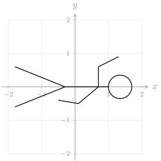
If you compare the two plots carefully you’ll see that he’s actually been reflected around the $y = x$ line. We can bring this about by simply switching all the $x$ and $y$ coordinates used to plot the picture. This corresponds to the following matrix multiplication:

\[\begin{bmatrix} 0 & 1 \\ 1 & 0 \\ \end{bmatrix} \begin{bmatrix} x \\ y \\ \end{bmatrix} = \begin{bmatrix} y \\ x \\ \end{bmatrix}\]

The matrix rows each explain how to make one output coordinate by mixing together the two input coordinates in different proportions. Here the proportions are quite extreme:

\[\begin{matrix} 0x & + & 1y & = & y \\ 1x & + & 0y & = & x \\ \end{matrix}\]

Let’s pick him up by doing an anticlockwise rotation. The recipe for such a matrix, with $\theta$ being the angle to rotate by, is:

\[\begin{bmatrix} \cos \theta & -\sin \theta \\ \sin \theta & \cos \theta \\ \end{bmatrix}\]

Remember how we figured out that when we operate on a complex number by multiplying it by another complex number $a + bi$, it works the same as a matrix acting on a vector:

\[\begin{bmatrix} a & -b \\ b & a \\ \end{bmatrix}\]

That’s the same thing! To ensure the matrix doesn’t change the size of the picture as well as rotating it, we have to observe the rule:

\[a^2 + b^2 = 1\]

which using $\cos$ and $\sin$ takes care of. The polar form of a complex number is related to the cartesian form by:

\[r e^{i\theta} = r \cos \theta + r i \sin \theta\]

So we’re setting $r = 1$, and so $a = \cos \theta$ and $b = \sin \theta$, and we get the rotation matrix.

I want to stand Stick Man back up so I’ll set $\theta = 90^\circ$ ($\pi/2$):

\[\begin{bmatrix} 0 & -1 \\ 1 & 0 \\ \end{bmatrix}\]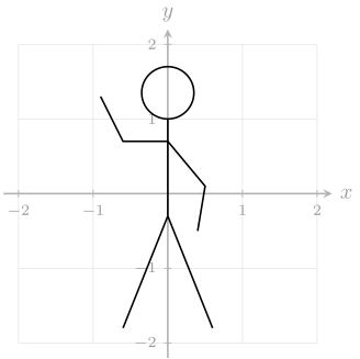

He’s not back quite how he was though, because he’s still reflected. Comparing him to how he was originally we’d say he’s reflected in the $y$-axis, which is the same as saying that the $x$-coordinate of all vectors has been sign-flipped. This is the combined effect of the two transformations we’ve applied. We did the reflection first, so that’s shown here inside parentheses acting directly on some vector to switch its coordinates, and to the result of that we apply the rotation:

\[\begin{bmatrix} 0 & -1 \\ 1 & 0 \\ \end{bmatrix} \left( \begin{bmatrix} 0 & 1 \\ 1 & 0 \\ \end{bmatrix} \begin{bmatrix} x \\ y \\ \end{bmatrix} \right) = \begin{bmatrix} 0 & -1 \\ 1 & 0 \\ \end{bmatrix} \begin{bmatrix} y \\ x \\ \end{bmatrix} = \begin{bmatrix} -x \\ y \\ \end{bmatrix}\]

But we could have bracketed it the other way and multiplied the two square matrices:

\[\left( \begin{bmatrix} 0 & -1 \\ 1 & 0 \\ \end{bmatrix} \begin{bmatrix} 0 & 1 \\ 1 & 0 \\ \end{bmatrix} \right) \begin{bmatrix} x \\ y \\ \end{bmatrix} = \begin{bmatrix} -1 & 0 \\ 0 & 1 \\ \end{bmatrix} \begin{bmatrix} y \\ x \\ \end{bmatrix} = \begin{bmatrix} -x \\ y \\ \end{bmatrix}\]

That is, the brackets are unnecessary, because matrix multiplication is associative. It is not commutative in general, so it matters what order we write the matrices in, but they can then be reduced down to a single matrix in stages, by combining any adjacent pair until there’s only one matrix left.

If you combine two linear operators in this way, the result is another linear operator. In this case we could probably have figured out the matrix to reflect $(x, y) \to (-x, y)$ but the point is, we can creatively combine rotations and other operators to produce a single matrix that does something interesting.

Let’s do something that is neither rotation nor reflection. Starting with the identity (or “do-nothing”) matrix, we can increase one of the diagonal entries, and shrink the other:

\[\begin{bmatrix} 2 & 0 \\ 0 & 0.5 \\ \end{bmatrix}\]

A matrix of this form, with any entries off the main diagonal set to zero, is called a diagonal matrix. As only the diagonal entries carry any information, you’ll sometimes see a matrix like this written in shorthand as $\operatorname{diag}(2, 0.5)$.

This will stretch the original (non-reflected) Stick Man along the $x$ axis but squish him along the $y$ axis:

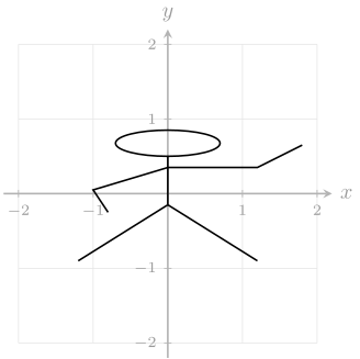
What if we wanted to do this kind of stretching and squishing along some angle, like $30^\circ$ clockwise? We don’t need to figure anything out ourselves. We just rotate Stick Man $30^\circ$ anticlockwise, then apply the above stretch/squish along the $x$/$y$ axis, then rotate him back again.

One thing I’m going to state without digging into (yet) is that once I’ve figured out the clockwise rotation, $R$, I can get the anticlockwise version very easily: it’s $R^\intercal$, the transpose. This is not a way to get the inverse of any matrix (and anyway, not all matrices have an inverse), but it always works for rotations and reflections.

Again, read any cluster of adjacent matrices from right to left to get the effective order they get applied in:

\[\begin{eqnarray} \begin{bmatrix} 0.87 & 0.5 \\ -0.5 & 0.87 \\ \end{bmatrix} \begin{bmatrix} 2 & 0 \\ 0 & 0.5 \\ \end{bmatrix} \begin{bmatrix} 0.87 & -0.5 \\ 0.5 & 0.87 \\ \end{bmatrix} &=& \begin{bmatrix} 0.87 & 0.5 \\ -0.5 & 0.87 \\ \end{bmatrix} \begin{bmatrix} 1.74 & -1 \\ 0.25 & 0.44 \\ \end{bmatrix} \\ &=& \begin{bmatrix} 1.64 & -0.65 \\ -0.65 & 0.88 \\ \end{bmatrix} \end{eqnarray}\]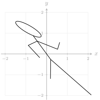

Such a combined matrix still has the effect of stretching or squishing along axes that are at right angles, but those axes don’t have to be aligned with our coordinate grid. If we twisted our coordinate grid around to aline with the this operator’s stretch/squish axes, then in that basis the operator would just be the original $\operatorname{diag}(2, 0.5)$.

The matrix has a characteristic pattern: the main diagonal can have any values, but the off-diagonal entries must match their diagonal opposites. Or to put it another way, the matrix must equal its own transpose: $M = M^\intercal$. This always happens with this kind of rotated-stretch/squish operator because of the ingredients it has to be composed from.

So if you spot a matrix that is equal to its own transpose, then you know two things:

• It works by picking out two orthogonal directions (not necessarily the basis directions) and scaling along them.
• There is a basis (aligned with those orthogonal scaling directions) in which it can be written as a diagonal matrix.

For such a matrix, certain vectors are special, being the ones that aren’t realigned by the transformation it performs. These are the orthogonal directions it purely scales along. Along all other directions, it also alters the alignment of vectors, because it scales their coordinates differently. The technical name for vectors that are not realigned by an operator is eigenvectors. They are like geometrical signposts or features of the operator that tell you “which way it is pointing”.

Also the observation that a matrix like this has orthogonal eigenvectors that can serve as a basis, and so we can always describe the same operator in that eigenbasis as a simple diagonal matrix, is known as the spectral theorem, although in the form we’ve stated it here, it’s the real version, while in QM we’ll need to generalise it a little to allow for complex scalars. Taking a symmetric matrix and splitting it into an equivalent sequence: rotate, diagonal matrix, un-rotate, is called spectral decomposition.

Why spectral? The word spectrum is often used to mean a single parameter, a control that can be slid from side to side to specify its value. But in science, it originates with Newton’s discovery that light can be separated into different frequencies. So a spectrum is a collection of parameters, in fact an infinite continuum of parameters. At each frequency, there is a number saying how powerful the light is. But we can have discrete spectra as well, though that’s still an infinite list of parameters. And finally, we could have a finite spectrum: a list of numbers. A diagonal matrix such as $\operatorname{diag}(2, 0.5)$ is entirely specified by a list of numbers. This is all it refers to in this context: noting that certain linear operators have a structure that means they can be described by a list of numbers, i.e. a spectrum.

But at this point these are all fancy names for thinking about how we can stretch a Stick Man.