Quantumania 5 - Geometry Strikes Back

Last time I got a little depressed to find that the cosy intuitive picture of vectors as arrows, living in the kind of geometry that fits in our heads, pretty much deserts us when dealing with complex vector spaces.

Coordinate-wise addition works exactly the same, and if we take each coordinate in cartesian form, $p + qi$, and split it into those two separate coordinates, addition still works exactly the same. But thinking geometrically, we don’t want to depend on the existence of a coordinate system. This urge to eradicate coordinates threatens to descend down into the complex plane itself. Who decided where the real and imaginary axes should be? Can we think of them also as an arbitrary choice?

Well, yes, in QM they effectively are, if we’re careful. First, in coordinate terms, we can state this precisely. If you have a state vector expressed in coordinates, you can multiply every single coordinate by the same unit complex number, that is, a phase factor, $e^{i\theta}$, and the resulting state vector describes exactly the same physical state. The overall phase of the state vector of an isolated system is completely irrelevant physically. So we kind of can say that you could tilt the real and imaginary axes of the complex plane, adjust all the complex coordinates accordingly, and still be describing the same physical state.

And crucially, this is in addition to the fact that its magnitude is always normalised to be $1$ (which is another way of saying that its magnitude is also irrelevant.)

We say that the states correspond to rays, which can be defined by the idea of an equivalence class over vectors: if two non-zero vectors $\vert \psi \rangle$ and $\vert\chi\rangle$ are colinear, they are equivalent, in that the thing they have in common is that they are examples of the same ray:

\[\vert \psi \rangle \sim \vert \chi \rangle \iff \vert \psi \rangle = c \vert \chi \rangle \quad \text{for some } c \in \mathbb{C} \setminus \{0\}\]

Notation decoder:

• The $\iff$ means “if and only if”, sometimes written as iff.
• The $\mathbb{C} \setminus {0}$ on the end there is defining the set of complex numbers except for zero.

You can’t scale a ray, and so you can’t make a ray “point in the opposite direction”. In a real vector space, you have to visualise them as lines extending both ways to infinity through the origin (and in a 2D complex vector space, as a certain kind of plane through the origin of a four-dimensional space… good luck with that). They have neither magnitude nor phase. All they have is alignment. These are what distinct states are actually represented by.

So if you scale the state vector by $e^{i\theta}$, it means the same thing physically. (If you scale it by a non-unit factor $r e^{i\theta}$, you’ll then need to normalise it by $1/r$, so you really just scaled it by $e^{i\theta}$.)

Now, given the apparent irrelevance of complex phase to the physical interpretation of the state, you could be forgiven for wondering why we have to use a complex vector space at all. It’s because of how states can be described as a linear composition of other states, and in that context, the full flexibility of complex scalars is required. It matters whether the two vectors being added point in opposite directions, because if they do, they will cancel out. And because the coordinates we scale by are complex, altering the relative phase of the components can affect the alignment of the resultant.

There is a commonly used visualisation that ties all these things together, called the Bloch sphere. But I’d advise caution: it can worsen any existing confusion instead of helping. Keep the following things in mind:

• It is not a way of visualising one vector, so much as a way of visualising how two orthonormal components can be scaled and summed to make one vector.
• The aim is to figure out what minimal independent parameters we really need, i.e. separately adjustable dials, avoiding the redundancy we’ve encountered with overall magnitude and phase being physically irrelevant.

Let’s start with the cartesian complex coordinates $a, b$, and eliminate the redundancy in stages:

\[\vert \psi \rangle = a \vert \alpha \rangle + b \vert \beta \rangle\]

We have to choose $a$ and $b$ so that the resultant is a unit vector, which means that $a$ and $b$ are not as independent as they look: once we’ve chosen $a$ we’re limited in what values we can give to $b$. We only really need to say how we’re going to “share” our unit of real magnitude between the two components: if $\vert a \vert$ increases, $\vert b \vert$ decreases, so really this is only one real parameter. Using trigonometry, we’re talking about a right-triangle with hypotenuse $1$, wedged inside the unit circle, so we can only change the angle $\theta$, and this alone determines the width of the adjacent side and the height of the opposite side:

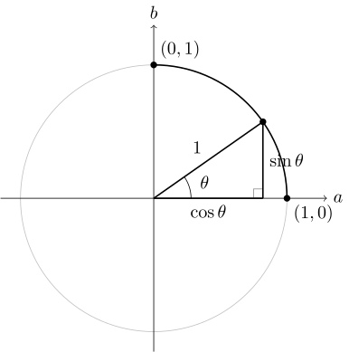
We could allow $\theta$ to have the full range $0 \leq \theta \lt 2\pi$ of an angle sweeping a circle, so that $\cos$ and $\sin$ can generate coordinates in all four compass directions and anything in between. But (for reasons that are about to become clear) we’re just interested in it being a kind of “balance knob” in the positive quadrant, so it only needs the range $0 \leq \theta \leq \pi/2$. When it’s $0$, it generates the coordinate pair $(1, 0)$, and when it’s $\pi/2$, it generates $(0, 1)$. Using any angle between, we can generate every allowed mixture.

So far we’ve got $\vert a \vert = \cos \theta$ and $\vert b \vert = \sin \theta$:

\[\vert \psi \rangle = \cos \theta \vert \alpha \rangle + \sin \theta \vert \beta \rangle\]

But that only lets us control the modulus of each coordinate. Then there’s the phases of the two components. This is what lets us access negative coordinates, of course, and is why we restricted the range of $\theta$ (otherwise we’d have two ways to represent the same state with different parameters, which is exactly the kind of redundancy we’re trying to stamp out.)

If we were to scale both $\vert \alpha \rangle$ and $\vert \beta \rangle$ by the same phase, the physical state being represented is unchanged. So really we only care about the difference between their phases. That is, we can let $\vert \alpha \rangle$ have phase angle $0$ (phase factor $1$), and only specify an adjustable phase $e^{i\phi}$ on $\vert \beta \rangle$, and allow the range of $\phi$ to sweep the full circle, $0 \leq \phi \lt 2\pi$:

\[\vert \psi \rangle = \cos \theta \vert \alpha \rangle + e^{i\phi} \sin \theta \vert \beta \rangle\]

We therefore have only two adjustable dials $\theta$ and $\phi$, instead of the four that were implied by $a$ and $b$ as independent complex coefficients, and no redundancy in terms of physical state representations: every state corresponds to a different pair of numbers, and vice versa.

The symbols we’ve chosen for these are not a coincidence, although to finish the picture in the standard way, we need to make one slight adjustment. These are the symbols for two angular coordinates in the global positioning system, albeit with some differences:

• $\theta$ - latitude, $0$ at the North Pole, $\pi$ at the South Pole, and therefore $\pi/2$ at the Equator. The symbol looks like a sphere with an equator around it - neat, huh? Specify a latitude and you’ve chosen a circle to travel around on as the Earth spins on its axis. Note that in geography we put the zero angle at the equator, but that would just make our formula look more messy for no particular reason. So we’ll ignore this difference.
• $\phi$ - longitude, the angle that sweeps around as the Earth rotates once every 24 hours, so it tells you where you are on your circle of constant latitude. Again, the symbol looks like the kind of curve you are choosing with this parameter.

These two parameters identify a point on the sphere, and that means we could identify states with points on the sphere. The other difference with our definition so far is that our $\theta$ has to range over $0 \leq \theta \leq \pi/2$, so the standard polar angle has twice the range we allow. No problem: we’ll convert down to our requirements by dividing $\theta$ by two:

\[\vert \psi \rangle = \cos \left( \frac{\theta}{2} \right) \vert \alpha \rangle + e^{i\phi} \sin \left( \frac{\theta}{2} \right) \vert \beta \rangle\]

But, I can almost hear you grumbling, what about the fact that at the poles there are infinitely many pairs of coordinates that map to the same point? When $\theta = 0$, we’re at the North Pole, and longitude $\phi$ becomes redundant. Same at $\theta = \pi$, the South Pole. But this redundancy only occurs at those two points, and they correspond to the trivial cases where the resultant vector is exactly $\vert \alpha \rangle$ or $\vert \beta \rangle$, and multiplying by a phase will either have no effect or will only change the overall phase, which is indeed physically redundant. Oh well, you can’t win them all, and you can’t map a sphere with a single coordinate system patch that has no singularities on it. Let’s sweep this under the Möbius carpet for now.

And there we have it: the Bloch sphere has coordinates that work similarly to the coordinates we use to map the globe, and the above formula converts them into Cartesian complex coordinates for making a linear combination of two orthogonal unit vectors.

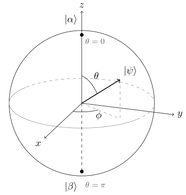
The immediately apparent danger with this is that it clearly shows $\vert \alpha \rangle$ and $\vert \beta \rangle$ as antipodes, at the North and South poles, as if they are vectors pointing in opposite directions, which would make them colinear, separated by a scale factor $-1$. But they are in fact orthogonal vectors in the state space.

But this is not just designed to confuse us. By eliminating the physical redundancy in the parameters, we’ve found a visual representation that maps directly to the physical interpretation in a specific and very important scenario: the spin of an electron. The spin is something that always has the same magnitude, but when we measure it, which we can only do by choosing an axis in space along which to measure, we find it points in one or the other direction along that axis.

We haven’t really touched on the dreaded measurement problem so I don’t want to labour this point. But for any state, there is an axis (if only we knew what it was) that is certain to produce a definite measurement outcome. We can say that this axis is characterised by a point on a sphere in 3D physical space, which we can specify with our two parameters (which is why mathematicians call the familiar globe a 2-sphere.)

So we can identify two orthogonal unit vectors in the state space with two opposing directions for the spin in physical space. Let’s relabel $\vert \alpha \rangle$ as $\vert u \rangle$ (for “up”) and $\vert \beta \rangle$ as $\vert d \rangle$ (for “down”).

When $\theta = 0$, the spin is up, and when $\theta = \pi$, the spin is down (and, as we grumbled, $\phi$ is meaningless). But by adjusting these parameters, we can build other pairs of antipodal points on the sphere, which also correspond to orthogonal unit vectors in the state space. And guess what: these are the actual directions in physical space. We are, as the Book says, “forced to resort to astonishment.”

The diagram of the sphere above anticipates this, labelling the cartesian 3D spatial directions. The up/down direction is labelled $z$ as you’d normally expect. We can find the two antipodes of the $x$ direction by setting latitude $\theta = \frac{\pi}{2}$ (the Equator) and making $\phi$ be either $0$ or $\pi$. Plug these into the Bloch formula and you have the orthogonal state vectors for “front” and “back”, expressed as a mixture of up and down:

\[\vert f \rangle = \frac{1}{\sqrt{2}}\vert u\rangle + \frac{1}{\sqrt{2}}\vert d \rangle \,\,\,\,\,\,\,\,\,\,\,\, \vert b \rangle = \frac{1}{\sqrt{2}}\vert u\rangle - \frac{1}{\sqrt{2}}\vert d \rangle\]

(Warning: $b$ was being used before as one of the cartesian coordinates of our linear combination, whereas here $\vert b \rangle$ is an entirely unrelated shorthand for “back”.)

These are exactly the same $\vert + \rangle$ and $\vert - \rangle$ mixtures we sketched way back on Monday, back when we were comfortably in denial about the involvement of complex numbers. But note that we were on perfectly safe ground: we got the right answer, but we were limited to finding the states representing only two of the three dimensions of physical space. Now we can find the $y$ directions, “right” and “left”, staying on the equator and letting $\phi$ be either $\pi/2$ or $3\pi/2$:

\[\vert r \rangle = \frac{1}{\sqrt{2}}\vert u\rangle + \frac{i}{\sqrt{2}}\vert d \rangle \,\,\,\,\,\,\,\,\,\,\,\, \vert l \rangle = \frac{1}{\sqrt{2}}\vert u\rangle - \frac{i}{\sqrt{2}}\vert d \rangle\]

The complex phase difference $i$ between the two components is what creates the extra degree of freedom, and a difference of phase between the two vector components is the only kind of phase ingredient we can specify with the Bloch coordinates.