Quantumania 7 - There's More Than One Thing in the Universe

I want to start talking about this stuff in the language of quantum computing. My motivation for this is straightforward: when you learn the basics of QM, you are like a baby that has just figured out how to reach out and grab a cup with one hand and slam it excitedly down on the table a few times in triumph at your achievement, spilling your drink everywhere. In contrast, people who work on quantum computing algorithms are like Penn & Teller, who can juggle a bowling ball, a bowling pin, a newly sharpened axe and an apple, and casually take a bite from the apple each time it lands in their right hand.

We’ve been considering systems that can be (in some sense) “measured” to produce a binary outcome. We’re going to refer to these from now on as qubits. As I complained the first time I used that word, we need to bear in mind that as systems described by complex 2-vectors, they have the ability to be measured along any axis in physical space, and we saw exactly how this flexibility is packed into the vector space by discovering the Bloch sphere, a method for describing the state of a qubit in terms of a chosen measurement axis in physical space, which is to say, in terms of a chosen orthonormal basis in state space.

Right at the very start I talked about how a system is always described by a state vector, and then I teased the idea that actually this is only true of an isolated system, which might be made up of subsystems. In fact I suggested that the only true example we have of an isolated system is the entire universe. So it’s high time we asked how this actually works, using qubits as building blocks.

Based on how things work in classical physics, we might take a couple of qubits and sit them side by side, and ponder that the state must surely be fully described by two state vectors, one for each qubit. Why would it be any other way? If we have $N$ particles, each needing some small number $k$ of variables to describe its state, then we need $kN$ variables altogether.

A one-qubit system can be analysed in terms of physical space by choosing a measurement axis, defining a North/South pole, and in terms of a state vector space that has two orthogonal unit vectors corresponding to the North and South poles. Any direction in physical space can be described by a scaled sum of those unit vectors. But given this chosen measurement axis, there are only two possible outcomes, which in accordance with qubit conventions we’re going to call $\vert 0 \rangle$ and $\vert 1 \rangle$. Those orthogonal basis vectors serve as ingredients that all states can be composed from.

In a two-qubit system, there are four possible measurement outcomes given choice of basis, a situation we can represent symbolically in a few ways. The most succinct is:

\[\vert 00 \rangle \,\,\,\,\,\, \vert 01 \rangle \,\,\,\,\,\, \vert 10 \rangle \,\,\,\,\,\, \vert 11 \rangle\]

The first digit indicates the measurement outcome of the first qubit, and so on. So the order is significant and we can’t for example treat $\vert 01 \rangle$ and $\vert 10 \rangle$ as the same state.

These are the basis vectors of a 4-dimensional state space. So the state of the two-qubit system $\vert \psi \rangle$ might be exactly aligned with one of these outcomes:

\[\vert \psi \rangle = \vert 01 \rangle\]

Or it could be that the state is such that all outcomes are equally likely:

\[\vert \psi \rangle = \frac{1}{2} \vert 00 \rangle + \frac{1}{2} \vert 01 \rangle + \frac{1}{2} \vert 10 \rangle + \frac{1}{2} \vert 11 \rangle\]

Note the normalisation factor: $(1/2)^2 = 1/4$, so this is a unit vector as required. Another possible state:

\[\vert \psi \rangle = \frac{1}{\sqrt{2}} \vert 00 \rangle + \frac{1}{\sqrt{2}} \vert 11 \rangle\]

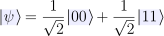
If this was the state, then a measurement of the first qubit would make it unnecessary to measure the second: we’d already know it, because the only states with a non-zero probability of being measured are the ones where the qubits are the same. Also, of course, we can create such superpositions except with a phase difference between the two terms, e.g.

\[\vert \psi \rangle = \frac{1}{\sqrt{2}} \vert 00 \rangle - \frac{i}{\sqrt{2}} \vert 11 \rangle\]

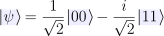
At first glance this might not seem so strange. We noted that classically speaking, if we have $N$ particles, each needing some small number $k$ of variables to describe its state, then we need $kN$ variables altogether. So it appears that here $k = 2$, and so for one qubit ($N=1$) we needed a 2-dimensional state space, and for two we need a 4-dimensional state space. So far, so classical. But if we add a third qubit:

\[\vert 000 \rangle \,\,\, \vert 001 \rangle \,\,\, \vert 010 \rangle \,\,\, \vert 011 \rangle \,\,\, \vert 100 \rangle \,\,\, \vert 101 \rangle \,\,\, \vert 110 \rangle \,\,\, \vert 111 \rangle\]

Now there are $2^3 = 8$ possible outcomes to each be represented by an orthonormal basis vector and thus a separate state vector coordinate in this basis. Classically we’d assume the states of the qubits to be independent, so requiring $2$ vector coordinates each, giving $2 \times 3 = 6$. Each qubit we add should mean we need another $2$ coordinates. But that’s not what happens in QM. Each qubit we add doubles the number of coordinates. As the number of qubits increases further, it starts to get really silly. A system with 10 qubits has 1024 possible outcomes. A system with 20, over a million outcomes. With 30, over a billion outcomes, over a billion dimensions to the state space, over a billion coordinates required to describe the state. At 300 qubits, we’d need many times more coordinates to represent the state than there are atoms in the observable universe. What is going on? Why do we need so much room in the description of the state?

When Dirac first realised this is how QM needed to work, he called the basic unit joint states direct product states. So the state $\vert 01 \rangle$ is in some sense the product of the separate (ordered) states $\vert 0 \rangle$ and $\vert 1 \rangle$, and can also be written:

\[\vert 01 \rangle = \vert 0 \rangle \otimes \vert 1 \rangle\]

Despite being described as a product, it is not commutative: swap the inputs and you get a different state vector in the combined state space. This is, as realised a few years later by von Neumann, the tensor product.

In the $\vert 0 \rangle, \vert 1 \rangle$ basis, we can describe any vector using coordinates that scale the two basis vectors. This is of course true of the basis vectors themselves, which we’ve already seen are represented in coordinates as the one-hot column vectors:

\[\vert 0 \rangle \equiv \begin{bmatrix} 1 \\ 0 \\ \end{bmatrix} \,\,\,\,\,\,\,\,\,\,\, \vert 1 \rangle \equiv \begin{bmatrix} 0 \\ 1 \\ \end{bmatrix}\]

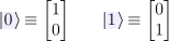
By the way, at this point the qubit notation practically invites us to get confused. The $0$ inside $\vert 0 \rangle$ is not playing any kind of arithmetic role. It’s just a label, an interpretation or meaning attached to a state vector. Feel free to mentally replace these labels with $\vert u \rangle$ or $\vert d \rangle$, or, even better, get in the habit of “tuning out” the state labels, and don’t mistake them for playing a directly numerical role here. Meanwhile, the numbers in the column matrix are actual numbers, and we’re going to do some (not at all taxing) arithmetic with them right now.

Once we switch to working in coordinates, $\otimes$ simply means to “multiply out” the coordinates:

\[\begin{bmatrix} a \\ b \\ \end{bmatrix} \otimes \begin{bmatrix} c \\ d \\ \end{bmatrix} = \begin{bmatrix} ac \\ ad \\ bc \\ bd \\ \end{bmatrix}\]

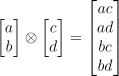
This is known as the Kronecker product, but the shared $\otimes$ symbol turns out to be quite appropriate, and we often refer this as the tensor product too. The output is a four-dimensional column vector. Also because every entry in the output is a simple product, $\otimes$ is evidently distributive over vector addition:

\[\vert \chi \rangle \otimes (\vert \psi \rangle + \vert \phi \rangle) = (\vert \chi \rangle \otimes \vert \psi \rangle) + (\vert \chi \rangle \otimes \vert \phi \rangle)\]

That is, we can “multiply out” tensor products. Similarly, applying some scalar factor $k$ to the tensor product is the same as applying it to either of the inputs:

\[k (\vert \psi \rangle \otimes \vert \phi \rangle) = (k \vert \psi \rangle) \otimes \vert \phi \rangle = \vert \psi \rangle \otimes (k \vert \phi \rangle)\]

We can check what the tensor product gives us when we apply it to all four possible combinations of the basis vectors in the two-qubit system:

\[\vert 00 \rangle = \vert 0 \rangle \otimes \vert 0 \rangle \equiv \begin{bmatrix} 1 \\ 0 \\ \end{bmatrix} \otimes \begin{bmatrix} 1 \\ 0 \\ \end{bmatrix} = \begin{bmatrix} 1 \\ 0 \\ 0 \\ 0 \\ \end{bmatrix}\] \[\vert 01 \rangle = \vert 0 \rangle \otimes \vert 1 \rangle \equiv \begin{bmatrix} 1 \\ 0 \\ \end{bmatrix} \otimes \begin{bmatrix} 0 \\ 1 \\ \end{bmatrix} = \begin{bmatrix} 0 \\ 1 \\ 0 \\ 0 \\ \end{bmatrix}\] \[\vert 10 \rangle = \vert 1 \rangle \otimes \vert 0 \rangle \equiv \begin{bmatrix} 0 \\ 1 \\ \end{bmatrix} \otimes \begin{bmatrix} 1 \\ 0 \\ \end{bmatrix} = \begin{bmatrix} 0 \\ 0 \\ 1 \\ 0 \\ \end{bmatrix}\] \[\vert 11 \rangle = \vert 1 \rangle \otimes \vert 1 \rangle \equiv \begin{bmatrix} 0 \\ 1 \\ \end{bmatrix} \otimes \begin{bmatrix} 0 \\ 1 \\ \end{bmatrix} = \begin{bmatrix} 0 \\ 0 \\ 0 \\ 1 \\ \end{bmatrix}\]

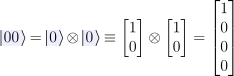
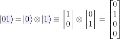
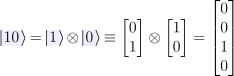
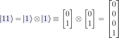
So this checks out: the four base states of the combined two-qubit system have the expected one-hot vector representations. But more generally, we can take the column 2-vectors of any pair of states $\vert \phi \rangle$, $\vert \chi \rangle$ for the two qubits considered separately, and multiply them out in the same way, and we’ll have the column 4-vector for the combined state that means “the first qubit is in state $\vert \phi \rangle$ and the second qubit is in state $\vert \chi \rangle$”.

But if these were the only states possible, we wouldn’t need a billion-dimensional space for a system of 30 qubits. There must be more to it.