Quantumania 18 - Mixed Messages

We’ve considered measurable things, such as which way something is pointing in space, and the framework we’ve given for that implied that the only kinds of physical measurement we can do involve measuring in one basis. That is, all the possible outcomes of the measurement correspond to orthogonal state vectors, giving us a very convenient basis in which to capture the state vector in coordinates, such that each coordinate gives us one of the outcomes.

Another way to write this is as follows. If $\vert M_n \rangle$ is the vector associated with the $n$-th measurement outcome, and clearly our state vector $\vert \psi \rangle$ can be thought of as a column vector written in the basis $\lbrace \vert M_1 \rangle, \vert M_2 \rangle \dots \rbrace$, then:

\[\langle M_n \vert \psi \rangle\]

in effect means “pluck the $n$-th coordinate out of $\psi$”.

Recalling that if you switch the labels on a bra-ket it’s the complex conjugate, and to convert the $n$-th coordinate into the probability of obtaining the $n$-th measurement outcome we need to multiply it by its own complex conjugate, that probability can be written:

\[\langle \psi \vert M_n \rangle \langle M_n \vert \psi \rangle\]

But we’ve written it in a way that doesn’t assume anything about a coordinate representation in any basis. We’re using operations with a geometrical meaning: the inner product of two vectors, which is invariant, completely independent of the choice of basis. We know our state vector could be described in the measurement basis, that is, there must be some column of complex coordinates $c_n$ such that:

\[\vert \psi \rangle = \sum_n \vert M_n \rangle c_n\]

And we can use the inner product to get those coordinates, $c_n = \langle M_n \vert \psi \rangle$. Substituting:

\[\vert \psi \rangle = \sum_n \vert M_n \rangle \langle M_n \vert \psi \rangle\]

In that expression our eye is naturally drawn to the familiar bra-ket pattern, which we should be in the habit of seeing as a scalar. So the expression inside the sum builds a vector that is colinear with $\vert M_n \rangle$, as that’s what we’re scaling. But let’s pull out this part by itself:

\[\vert M_n \rangle \langle M_n \vert\]

We could call this a ket-bra, I guess? Nobody does though. Given that the bra-ket’s official name is the inner product, it’s easy to remember the ket-bra’s official name, the outer product. The role played by this object in our example is to operate on a vector to product another vector, and so it’s an operator and can be represented by a matrix. In fact, if we have a column vector representing $\vert M_n \rangle$, and we use the hermitian conjugate to get a row vector representing $\langle M_n \vert$, writing them side-by-side in ket bra order is simply matrix multiplication:

\[P_n = \vert M_n \rangle \langle M_n \vert \equiv \begin{bmatrix} a \\ b \end{bmatrix} \begin{bmatrix} a^* & b^* \end{bmatrix} = \begin{bmatrix} a a^* & a b^* \\ b a^* & b b^* \end{bmatrix}\]

So for the basis vectors in the measurement basis:

\[P_1 = \vert M_1 \rangle \langle M_1 \vert \equiv \begin{bmatrix} 1 & 0 \\ 0 & 0 \end{bmatrix} \quad \quad P_2 = \vert M_2 \rangle \langle M_2 \vert \equiv \begin{bmatrix} 0 & 0 \\ 0 & 1 \end{bmatrix}\]

These are called projection operators, because when applied to a vector $\vert \psi \rangle$, they project it onto the vector they were built from. $P_1$ flattens a vector into alignment with $\vert M_1 \rangle$, making the component vector of $\vert \psi \rangle$ along $\vert M_1 \rangle$, or $c_1 \vert M_1 \rangle$ where $c_1$ is the first coordinate of $\vert \psi \rangle$ in the $M$ basis. So if used like this:

\[\langle \psi \vert P_n \vert \psi \rangle = \langle \psi \vert M_n \rangle \langle M_n \vert \psi \rangle = c_n^* c_n\]

So we go straight to the probability of obtaining the $n$-th measurement outcome from state $\langle \psi \vert$. Why bother to think of the middle operator as new type of thing? Because this allows us to generalise the idea of a measurable outcome to include non-orthogonal possibilities. Measuring equipment isn’t always as ideal as we might imagine.

Even so, we can see how this looser way of defining measurement can be applied if we imagine a scenario that is still idealised, but in a different way to usual. Suppose Alice is going to receive (from Bob, of course) a qubit and all she knows is that its state is going to be either $\vert 0 \rangle$ or $\vert \mathbb{+} \rangle$. That is, either a basis state of the Z basis, or a basis state of the X basis. Welcoming back our old friend (don’t worry, there’s a whole new diagram coming up):

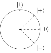
These two possibilities are not orthogonal. They’re at $45^\circ$ to one another. Each is a basis vector of one basis that can be expressed as a balanced superposition of the other basis.

If Alice measures in the Z basis she might find $\vert 1 \rangle$. As she knows Bob definitely didn’t send her that, she can conclude he definitely sent $\vert \mathbb{+} \rangle$ and it just flipped randomly into the $\vert 1 \rangle$ state. If he’d sent the other option, $\vert 0 \rangle$, she would have measured that with certainty, because it’s a basis vector of the basis she’s measuring in.

But if she finds $\vert 0 \rangle$, what does that tell her? Bob could have sent her $\vert 0 \rangle$, but equally he could have sent $\vert \mathbb{+} \rangle$ and it flipped into $\vert 0 \rangle$, as it randomly might. She could reason in much the same way about a measurement on the X basis. Whichever basis she chooses to measure in, the outcome is certain for one of the possibilities, occurring half the time (assuming Bob makes an unbiased random choice of what to send), and “Who knows?” for the other half.

The only way to improve on this is to make a trade-off: to accept getting a “Who knows?” answer more than half the time, but in exchange sometimes getting an absolutely certain answer for whichever qubit Bob sends. Mathematically the core of this is the orthogonal complement.

To picture this, think of a plane surface, orientated at some interesting angle. Then think of light rays shining on it so they are perfectly perpendicular to the plane. Now imagine a stick attached to the plane and sticking out from it. If the stick is itself perpendicular to the plane it won’t cast a shadow, because it’s in line with the light rays. But if the stick is tilted away from the perpendicular, it will cast a shadow. The shadow is the stick’s component in the plane.

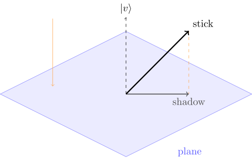
We can think of this as a 3D vector space if we visualise the origin as the point where the stick is attached to the plane. How can a plane exist in a vector space? Easy: it’s a set of vectors. The plane is a 2D subspace of the 3D space, containing all the vectors that lie in the plane.

We can turn the stick into the shadow by applying a projection operator that flattens 3D vectors into that 2D subspace. To construct that operator, suppose we know the vector $\vert v \rangle$ that is normal (orthogonal) to the plane, that is, it’s orthogonal to any vector lying in the plane. This is the vector that wouldn’t cast any shadow. Then we work out this operator:

\[I - \vert v \rangle \langle v \vert\]

It’s the projection operator on to $\vert v \rangle$ subtracted from the identity operator. So if we represent all this in coordinates such that $\vert v \rangle$ is the first basis vector:

\[\begin{bmatrix} 1 & 0 & 0 \\ 0 & 1 & 0 \\ 0 & 0 & 1 \\ \end{bmatrix} - \begin{bmatrix} 1 & 0 & 0 \\ 0 & 0 & 0 \\ 0 & 0 & 0 \\ \end{bmatrix} = \begin{bmatrix} 0 & 0 & 0 \\ 0 & 1 & 0 \\ 0 & 0 & 1 \\ \end{bmatrix}\]

The resulting matrix very clearly discards the first coordinate (the $\vert v \rangle$ direction) but retains the information from the other two (the plane), so flattens whatever vector it applies to into its shadow on the plane. And if applied a second time to that shadow, it will have no effect. The shadow exists in the 2D plane that is represented by the $2 \times 2$ square matrix in the lower right, which looks uncannily like the 2D identity matrix, because it is. To qualify as a projection operator, we only require that an operator is:

• hermitian (self-adjoint): $P^\dagger = P$
• idempotent: $P^2 = P$ (if applied a second time, it makes no difference, the damage is done.)

Now, in our example with qubits the space is two dimensional, so projection operators can only project onto lines, not planes.

\[\begin{bmatrix} 1 & 0 \\ 0 & 1 \\ \end{bmatrix} - \begin{bmatrix} 1 & 0 \\ 0 & 0 \\ \end{bmatrix} = \begin{bmatrix} 0 & 0 \\ 0 & 1 \\ \end{bmatrix}\]

So in 2D, the orthogonal complement of a vector is not a plane, it’s just another vector, although it is orthogonal to the original. But I wanted to get across the general idea as it pertains to higher dimensional vector spaces because that’s what we’re dealing with when we have more than one qubit.

Also, bear in mind that the kind of measurement we’re going to talk about next makes use of orthogonal complements to projection operators, which are themselves projection operators, and yet the official term “projective measurement” is reserved for the kind of measurement we’ve previously talked about, where we choose a basis to measure in, and the probabilities of obtaining the outcomes are found by projecting the state vector onto the basis vectors.

Back to Alice and Bob. Alice wants three measurement outcomes: two are definite answers: $\vert 0 \rangle$ or $\vert \mathbb{+} \rangle$, and the other is “don’t know.” It’s okay if she gets a lot of don’t-knows, as long as she never gets a confidently wrong answer.

By sending the qubit through certain purely unitary transformations, it is possible to effectively send it into the path of three detectors, each of which does an ordinary projective measurement (that is, measuring in a specific basis just as we’ve always talked about), but only one of the three detectors will actually detect something, because although we can’t say anything for sure about how the qubit travels to its destination, it ultimately “collapses” to one of the three possible destinations. Alice makes it so that one of the detectors has zero probability of detecting something if the input qubit was $\vert 0 \rangle$, another has zero probability for $\vert \mathbb{+} \rangle$, and the third mops up the remaining probability.

More precisely, the first detector’s probability of firing for a qubit in state $\vert \psi \rangle$ is:

\[\langle \psi \vert E_1 \vert \psi \rangle\]

where

\[E_1 \propto I - \vert 0 \rangle \langle 0 \vert\]

(Note that it’s proportional-to, rather than equal-to: there would be an overall scaling factor to make sure the probabilities add to $1$.)

The projection $E_1$ obliterates any component in the $\vert 0 \rangle$ direction. If the qubit is exactly $\vert 0 \rangle$, it has a zero-length shadow in this projection. There’s a similar $E_2$ that obliterates $\vert \mathbb{+} \rangle$. Finally, the don’t-know detector is just:

\[E_? = I - (E_1 + E_2)\]

It’s the complement of the sum of the other two complements: it throws away that which would cause the either of the other two to cast a shadow.

So Bob sends $\vert 0 \rangle$, detector 2 is the only one that definitely won’t fire. If he sends $\vert \mathbb{+} \rangle$, detector 1 cannot fire. Either way, detector 3 always has a probability of firing, so Alice will get a lot of don’t-knows. But if detector 1 fires, she knows for absolute certain that Bob sent $\vert 0 \rangle$, and if 2 fires she knows he sent $\vert \mathbb{+} \rangle$.