Quantumania 20 - Disentanglement

QM says the state of an isolated physical system is a well-defined thing, which I’ve characterised as sharp and definite, rather than blurry and uncertain, and which we’ve found two ways to represent: a vector in the state space, or a projection operator on that state space:

\ket{\psi} \quad \iff \quad \ket{\psi} \bra{\psi}

We can use the measurement operator for some measurement outcome (which can be as simple as the projection operator for the corresponding post-measurement state) to find the probability of an outcome, but that’s all. This implies some intrinsic uncertainty in how the universe works, sometimes called ontological probability, because the probability is aspect of the world, rather than just being due to our own lack of knowledge, which would be epistemic probability. If we attempt to measure some property, and the present state is not one of the post-measurement states associated with that property, we will nevertheless get a definite answer corresponding to one of the property’s post-measurement states, and it seems that nature chooses that answer at random. This is, in a sense, our own fault for asking the wrong question.

But the moment we measure an isolated system, it ceases to be isolated. Indeed, you could say that it never was isolated, as we were there the whole time too, along with the measuring equipment, all just subsystems of some larger system. This led us to consider composite state spaces accessed via the tensor product, which in turn led to the awkward realisation that sometimes the definite state of the composite system did not contain definite states for its subsystems. Only if the composite system is in a product state, meaning the tensor product of the states of the subsystems, can we regard the subsystem as having definite states of their own. To keep it much simpler than trying to model the state of ourselves, we’ll stick to just two qubits:

\ket{0} \otimes \ket{1} = \ket{01}

This is a product state, and is equivalent to saying that the first qubit is in $\ket{0}$ and the second is in $\ket{1}$ , so they can be thought of as possessing their own states. But this is a vector space; the sum of two vectors is also a vector, and so is also a physically real state, such as:

\frac{\sqrt{3}}{2} \ket{01} - \frac{1}{2} \ket{10}

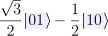
It can’t be rewritten as a product, in any basis. It’s inherently the sum of two product states. It is possible for you to know exactly the state this whole system was prepared in, and yet still not know what state the individual qubits are in, not because of epistemic uncertainty, but because the two qubits don’t have a state of their own. There is nothing certain for you to know. The probability of measuring $\ket{01}$ is $3/4$ , and there’s a $1/4$ chance of measuring $\ket{10}$ . This means that if you only measured the first qubit, $3/4$ times it’s $\ket{0}$ and $1/4$ it’s $\ket{1}$ .

Here’s where the idea of a mixed state really becomes useful. We introduced it by considering boring old epistemic uncertainty, a coin flip whose result Bob doesn’t know. But we can use exactly the same approach to represent something like the actual state of one of the individual qubits, or the closest thing it has to a state. Its state is intrinsically mixed, in reality itself, not just in our minds because we lack information. The mixed description is all the information there is in the world about that one qubit.

We know what that mixed state would look like for the first qubit as a matrix, expressed in the $Z$ basis, because we already worked out the probabilities:

\begin{bmatrix} \frac{3}{4} & 0 \\ 0 & \frac{1}{4} \end{bmatrix}

But this is only obvious because it’s a particularly simple setup. There is a proper way of getting from the density operator of a joint system to the density operator of one of its component subsystems that works even when the answer isn’t obvious. Our combined two-qubit system’s vector space is spanned by the usual basis vectors:

\lbrace \, \ket{00}, \ket{01}, \ket{10}, \ket{11} \, \rbrace

These are shorthands: $\ket{01} = \ket{0} \otimes \ket{1}$ and so on. There is a corresponding bra-space:

\lbrace \, \bra{00}, \bra{01}, \bra{10}, \bra{11} \, \rbrace

These are operators that act on a ket to produce a scalar, the inner product. Or we can write them in reverse as a ket-bra to make all the elementary projection operators (or in matrix form, matrices whose entries are all zero except for a single $1$ , which can be scaled and added to make any matrix.)

Through the tensor product, the parts of an operation related to one subsystem “find each other” and act independently. We saw exactly this when we applied the Hadamard operator $H^{\otimes n}$ to a whole register of $n$ qubits: it’s the same as applying Hadamard to each qubit individually. So these are equivalent:

\ket{i}\bra{k} \otimes \ket{j}\bra{l} = \ket{ij} \bra{kl}

So even if we aren’t certain of our joint two-qubit system’s state, and we have to describe it as a density operator rather than a pure state, that’s fine:

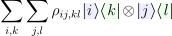
\sum_{i,k} \sum_{j,l} \rho_{ij,kl} \ket{i}\bra{k} \otimes \ket{j}\bra{l}

Here the $i$ , $j$ , $k$ and $l$ indices range over $\lbrace 0, 1 \rbrace$ , so they are the usual qubit basis state labels. Thus $\rho_{ij,kl}$ symbolises the 16 coefficients of the joint state’s density matrix $\rho$ , each giving a weighting to the tensor product of two single-qubit density operators. $i$ and $j$ label the kets, while $k$ and $l$ label the bras.

The exact way we’ve split the indices into different summations carries a significance, even though we could have written them many different ways. Ultimately we need all 16 combinations of the possible index values. But it makes sense to bunch them by which subsystem (qubit) they are driving. To see why, check out the almighty mess we get when we tabulate all the terms of the above sum:

\begin{matrix} & k=0, l=0 & k=0, l=1 & k=1, l=0 & k=1, l=1 \\ i=0, j=0 & \rho_{00,00} \ket{0}\bra{0} \otimes \ket{0}\bra{0} & \rho_{00,01} \ket{0}\bra{0} \otimes \ket{0}\bra{1} & \rho_{00,10} \ket{0}\

In each cell we write both the first and second qubit’s ket-bra, stitched together with the tensor product, and also scaled by the coefficient $\rho_{ij,kl}$ that would appear in the density matrix. $i$ and $j$ drive the rows, whereas $k$ and $l$ drive the columns.

It’s tricky to spot any pattern to it, but the way we grouped the summation variables doesn’t follow this ket/bra, row/column picture, and this is deliberate:

\sum_{i,k} \sum_{j,l}

Instead, it divides the labels according to subsystem: $i$ and $k$ produce the first qubit, $\ket{i}\bra{k}$ , whereas $j$ and $l$ produce the second, $\ket{j}\bra{l}$ .

The first qubit’s four basis states each relate to one of four quadrants of the table, visited in turn by the $\sum_{i,k}$ summation. The second qubit lives inside each quadrant as its four entries, visited by $\sum_{j,l}$ . Breaking it down into these quadrants and ignoring the details of the second qubit:

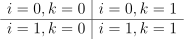
\begin{array}{c|c} i=0, k=0 & i=0,k=1 \\ \hline i=1, k=0 & i=1,k=1 \\ \end{array}

So there’s a hierarchy to it: the outer structure of quadrants describing the first qubit, the inner entries of each quadrant describing the second qubit. To distil it down to a $2 \times 2$ density matrix for the first qubit, we just need “blur our eyes”, turning the details of each quadrant into a single number. This is what the trace does, but here we’re applying it separately to each quadrant, and it’s called the partial trace:

\sum_{i,k} \sum_{j,l} \rho_{ij,kl} \ket{i}\bra{k} \cdot \operatorname{Tr} \Big( \ket{j}\bra{l} \Big)

Recall that $\ket{j}$ , being a basis vector, is a one-hot column. The outer product $\ket{j}\bra{l}$ in matrix form only ever has $1$ in a single entry, the rest being $0$ , and this single $1$ will only sit on the main diagonal if $j = l$ . This means that the trace is $1$ if $j = l$ and is $0$ otherwise, and further means that any term in our summation where $j \ne l$ will vanish. This gets rid of half the terms automatically.

Now, if you’re familiar with tensors as they appear in classical physics, you may be wondering why this isn’t just referred to as contraction, and I think you have a point! It is literally just an example of that. QM has its own terminology. Also, the hierarchical arrangement of the two subsystems is completely arbitrary, a byproduct of using matrix notation, and obscures more than it illuminates in my opinion. We don’t have to do it this way.

Not yet regretting the time you've spent here?