Quantumania 19 - Disappear With Trace

Last time we discovered projection operators, starting with the ket-bra or outer product:

\ket{\phi} \bra{\phi}

which operates on a vector $\ket{\psi}$ by projecting it onto $\ket{\phi}$ , i.e. scaling $\ket{\phi}$ by the inner product $\braket{\phi}{\psi}$ :

\ket{\phi} \braket{\phi}{\psi}

It may have occurred to you that such an operator can be thought of as an alternative representation of $\ket{\phi}$ . Rather than representing states as vectors in a vector space, perhaps we could instead represent them with operators acting on that vector space. This is appealing in that it means we represent everything through operators: states, transformations, measurements.

The downside is that it seems a little wasteful when you think about the numerical description of a qubit state in some basis as now requiring four numbers instead of two. But consider also that if we take a representation of $\ket{\phi}$ in some basis as having two coordinates $(\phi_1, \phi_2)$ , then the outer product produces a matrix:

\begin{bmatrix} \phi_1 \\ \phi_2 \end{bmatrix} \begin{bmatrix} \phi_1^* & \phi_2^* \end{bmatrix} = \begin{bmatrix} \phi_1 \phi_1^* & \phi_1 \phi_2^* \\ \phi_2 \phi_1^* & \phi_2 \phi_2^* \end{bmatrix}

The diagonal elements are always real, being the modulus squared of some complex number. Furthermore, assuming the basis is aligned with the eigenvectors of some observable, they are the probabilities of obtaining distinguishable measurement outcomes. Also they are all such probabilities, so they must sum to $1$ .

We’ve talked before about state vectors needing to be unit vectors so that when we interpret their coordinates as complex amplitudes, and take the modulus-squared, we get probabilities. By switching to projection operators as our states, we can replace that requirement by instead saying that the sum of the diagonal entries of the state’s projection operator must be $1$ . This aspect of a matrix is important enough to have a name, the trace, $\operatorname{Tr}(M)$ . When we think about matrices we can remember it simply as the sum of the diagonal entries. But perhaps surprisingly, it does not depend at all on our choice of basis. This means we’re not merely talking about the trace of a matrix specific to some numerical representation; we’re talking about the trace of an operator, an invariant basis-independent fact.

To see why, albeit it in a rather laborious way to begin with, recall that to convert a matrix to another orthogonal basis is simply to place it in the sandwich of rotation and un-rotation, $U M U^{-1}$ . The rotation takes the form:

U = \begin{bmatrix} x & -y^* \\ y & x^* \end{bmatrix} \quad \text{where } \vert x \vert^2 + \vert y \vert^2 = 1

That restriction on the sum of the squares is equivalent (in real vector spaces) to saying:

x = \cos \theta \quad \quad \quad y=\sin \theta

but we can put that out of our minds. More importantly, the inverse $U^{-1}$ is the adjoint $U^\dagger$ . Let’s make the basis-conversion sandwich around some matrix $M$ with any old entries:

M = \begin{bmatrix} j & k \\ l & m \end{bmatrix}

and multiply it on the left and then on the right:

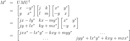
\begin{eqnarray*} M' &=& U M U^\dagger \\ &=& \begin{bmatrix} x & -y^* \\ y & x^* \end{bmatrix} \begin{bmatrix} j & k \\ l & m \end{bmatrix} \begin{bmatrix} x^* & y^* \\ -y & x \end{bmatrix} \\ &=& \b

I haven’t bothered to write in the off-diagonal entries at the end because we only want the trace, $\operatorname{Tr}(M')$ , so we add the main diagonal entries:

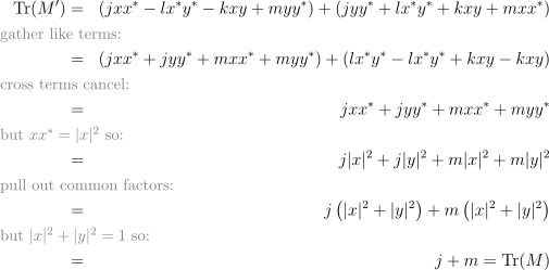
\begin{align*} \operatorname{Tr}(M') &=& \left( jxx^* - lx^*y^* - kxy + myy^* \right) + \left( jyy^* + lx^*y^* + kxy + mxx^* \right) \\ \shortintertext{\small\color{gray}gather like terms:} &=& \left(

The trace is unaffected by the change of basis. It is a fact about the operator described by the matrix, not merely a fact about the specific representation of that operator as a matrix in a particular basis.

Though there’s actually a much simpler way to reach this conclusion. Never mind rotations, consider any three matrices being multiplied together (again we only need the main diagonal entries):

\begin{bmatrix} p & q \\ r & s \end{bmatrix} \begin{bmatrix} a & b \\ c & d \end{bmatrix} \begin{bmatrix} j & k \\ l & m \end{bmatrix} = \begin{bmatrix} paj + qcj + pbl + qdl & \dots \\ \dots & kar +

Fine. But what do we get if we cycle the three inputs around so the first one moves to third place, second becomes first and third becomes second?

\begin{bmatrix} a & b \\ c & d \end{bmatrix} \begin{bmatrix} j & k \\ l & m \end{bmatrix} \begin{bmatrix} p & q \\ r & s \end{bmatrix} = \begin{bmatrix} paj + pbl + kar + mbr & \dots \\ \dots & qcj +

All the same terms are there, just switched around a bit, but that won’t affect the trace. So for any matrices $A, B, C$ :

\operatorname{Tr}(ABC) = \operatorname{Tr}(BCA)

This is the cyclic property of the trace. And therefore, as $U^\dagger U=I$ :

\operatorname{Tr}(U M U^\dagger) = \operatorname{Tr}(M U^\dagger U) = \operatorname{Tr}(M)

So now we’ve got two interesting facts about traces, in addition to the QM rule that for a projection operator $P$ representing a state, $\operatorname{Tr}(P) = 1$ . But we’re still waiting for the states-as-operators idea to really earn its keep by doing something new.

Okay, new scenario. Alice is sending Bob a qubit, and it’s either $\ket{0}$ or $\ket{1}$ , and she flips a coin to decide which. So is this a description of the state of the qubit?

\ket{+} = \frac{1}{\sqrt{2}} \Big( \ket{0} + \ket{1} \Big)

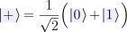
Nope. That’s a qubit state that Alice is definitely not going to send. All the way back at the start we swore never to be wishy washy and always remember that a state is a sharply defined arrow, and if you think of it as a superposition that’s a matter of interpretation. What we have here is sometimes called classical uncertainty. Put more simply, we know Alice is going to send one of two states, we don’t know which one, but we know they’re equally likely.

We can represent this state of knowledge (which is not the same thing as a state as we’ve been using that term so far) by weighting each state projection operator by its probability and adding the results:

\frac{1}{2} \ket{0} \bra{0} + \frac{1}{2} \ket{1} \bra{1} \equiv \begin{bmatrix} \frac{1}{2} & 0 \\ 0 & 0 \end{bmatrix} + \begin{bmatrix} 0 & 0 \\ 0 & \frac{1}{2} \end{bmatrix} = \begin{bmatrix} \frac

We can see that this is entirely different from the projection operator for $\ket{+}$ :

\ket{+}\bra{+} \equiv \begin{bmatrix} \frac{1}{\sqrt{2}} \\ \frac{1}{\sqrt{2}} \end{bmatrix} \begin{bmatrix} \frac{1}{\sqrt{2}} & \frac{1}{\sqrt{2}} \end{bmatrix} = \frac{1}{2} \begin{bmatrix} 1 & 1 \

So a matrix can describe our state of knowledge when it has some uncertainty about it, and in this case it’s a different thing from the so-called quantum uncertainty we hear about. There is a fact in the world, and Alice knows that fact, but Bob doesn’t. Alice and Bob would each make a different matrix to describe their own state of knowledge.

Alice would describe her state of knowledge with a pure state, a projection operator that is equivalent to a definite state vector. Bob would describe his state of knowledge with a mixed state (in this context a somewhat misleading term), which is the sum of all the possible pure state matrices, each weighted by its probability. The collective term for these is a density operator, after the classical concept of a probability density function, although it’s more common to hear the matrix representation of such an operator referred to as a density matrix.

But there’s a much more interesting application of these ideas, one which ties together much of the themes we’ve been wrestling with, even the dreaded measurement problem.

Not yet regretting the time you've spent here?